Basic splash usage
Simple two column plot
Once you have successfully compiled splash with a read data file that will read your data format, splash is invoked with the name of the data file(s) on the command line, e.g.
splash myrun*.dat
dprice$ splash -magma minidump.00001
    _                                                 _
   (_)   _               _           _         _     (_)_
      _ (_)    ___ _ __ | | __ _ ___| |__     (_)   _  (_)
   _ (_)  _   / __| '_ \| |/ _` / __| '_ \       _ (_)
  (_)  _ (_)  \__ \ |_) | | (_| \__ \ | | |  _  (_) _
      (_)  _  |___/ .__/|_|\__,_|___/_| |_| (_)  _ (_)
          (_)  (_)|_| (_) (_)  (_)(_) (_)(_) (_)(_)

  ( B | y ) ( D | a | n | i | e | l ) ( P | r | i | c | e )

...etc...
 You may choose from a delectable sample of plots
-------------------------------------------------------
  1) x                     7) particle mass
  2) y                     8) B\dx
  3) z                     9) B\dy
  4) h                    10) B\dz
  5) \gr                  11) div B
  6) T
-------------------------------------------------------
 12) multiplot [  4 ]      m) set multiplot
-------------------------------------------------------
 d(ata) p(age) o(pts) l(imits) le(g)end h(elp)
 r(ender) v(ector) x(sec/rotate) s(ave) q(uit)
-------------------------------------------------------
Please enter your selection now (y axis or option):
The simplest plot is of two quantities which are not both coordinates. For example, to plot density vs smoothing length, type
Please enter your selection now (y axis or option): 5
(x axis) (default=1): 4
 Graphics device/type (? to see list, default /xwin): /xw
The default= refers to the default value assigned if you just press
the return key. The last prompt asks for the device to which output
should be directed.
Hint
A full list of available graphics devices is given by typing ? at the prompt.
Some of the most useful devices are given in Commonly used graphics devices available in giza. In the above we have selected the X-window driver which means that the output is sent to the screen (provided X-windows is running), as demonstrated in the screenshot shown in Fig. 1.
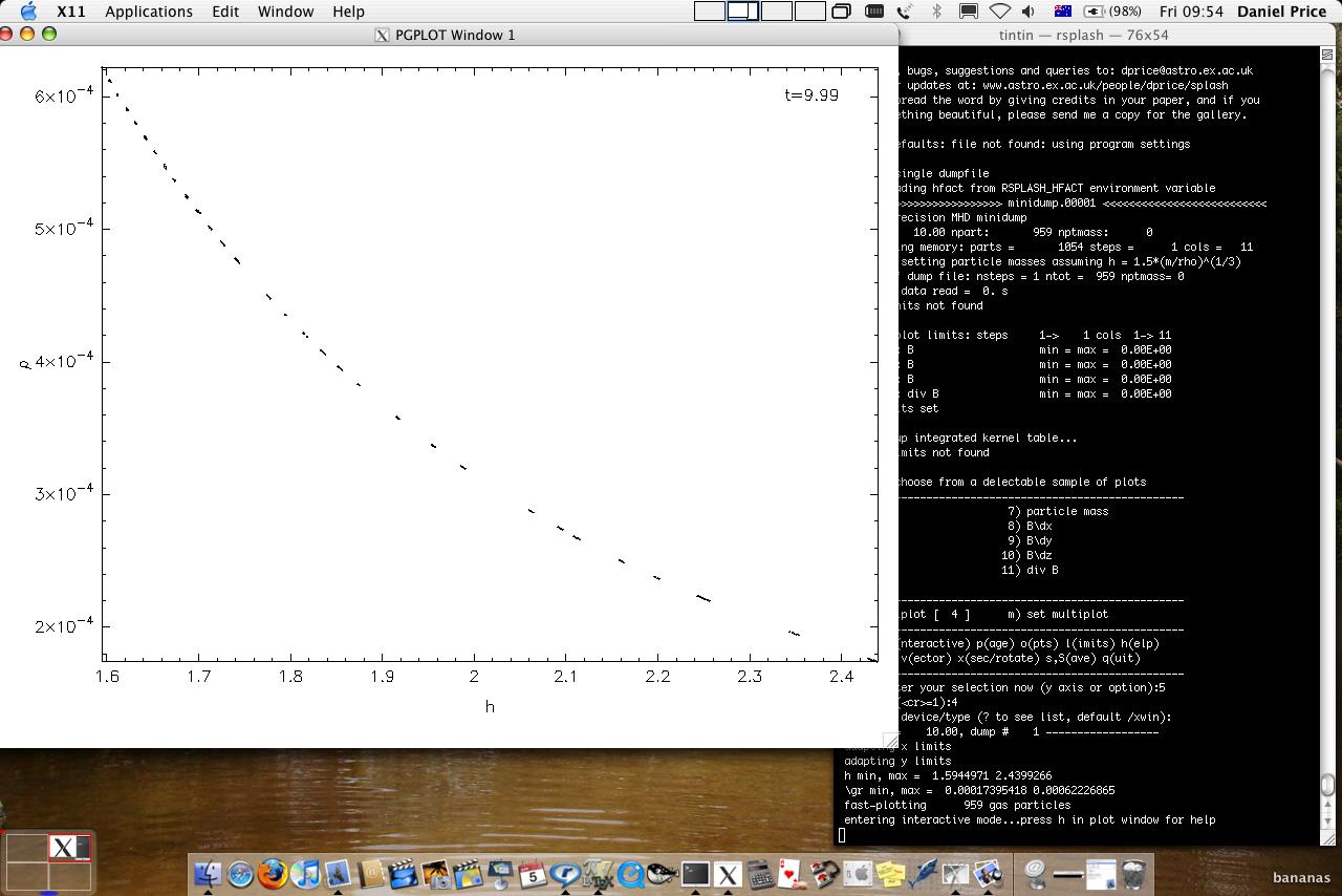
Fig. 1 Screenshot of simple two column plot to an X-window
|
X-Window (interactive) |
|
Portable Network Graphics (bitmap) |
|
Encapsulated postscript (one file per page) |
|
Scalable Vector Graphics |
|
|
null device (no output) |
|
|
Postscript (all pages in one file) |
|
mpeg4 animation (requires ffmpeg) |
Interactive mode
Many useful tasks can now be achieved by moving the mouse to the plot window and selecting areas or pressing keystrokes – this is Interactive mode. Most useful are:
press
lwith the mouse over the colour bar for a log axisato adapt the plot limits (with mouse on the colour bar, inside the plot, or positioned next to the x or y axes)left clickto select an area with the mouse andclickto zoomleft clickon the colour bar to change the rendering limitsspaceto skip to the next file (right clickorbto go back)-or+to zoom in or outEnterfor Hollywood modeoto recentre the plot on the originrto refresh the plot (e.g. after changing the window size)gto plot a line and find its gradientmorMto change the colour mapfto flip the rendering to the next quantity<,>,{,}and/,\to rotate particles around z, y and x axes, respectivelyGto move the legendctrl-tto annotate with textbackspaceto delete annotationsin the plot window to save changes between timesteps, otherwise the settings will revert when you move to the next timestep.qin the plot window to quit the plotting window and return to the menuqagain from the splash main menu to quit splash altogether.hin the plot window for the full list of commands
On particle plots you can additionally:
select an area and press
0-9to colour particles (particle colours stick between plots, so you can use this to find particles with unusual parameters)select an area and press
0to hide selected particlesmove the mouse over a particle and press
cto see the size of the smoothing circle for that particle
These tasks can also be achieved non-interactively by a series of
text-based Menus (see Changing plot settings). For example limits changing options are contained in the
(l)imits menu, so to manually set plot limits we would type l from
the main menu, then 2 for option 2 (set manual limits) and follow the
prompts to set the limits for a particular data column.
See also (i)nteractive mode.
Rendered plots
A more complicated plot is where both the \(x-\) and \(y-\) axes refer to coordinates. For example
Please enter your selection now (y axis or option):2
(x axis) (default=1): 1
(render) (0=none) ([0:11], default=0):5
(vector plot) (0=none, 8=B) ([0:8], default=0):0
Graphics device/type (? to see list, default /xwin): /xw
You can produce the same graph without answering prompts using:
splash -y 2 -x 1 -r 5 -dev /xw minidump.00001
or, since the other options are default anyway, simply:
splash -r 5 minidump.00001
Notice that in this case that options appeared for rendered and vector
plots. Our choice of 5 at the (render) prompt corresponds to column 5,
which in this case is the density, producing the plot shown in the
screenshot in Fig. 2.
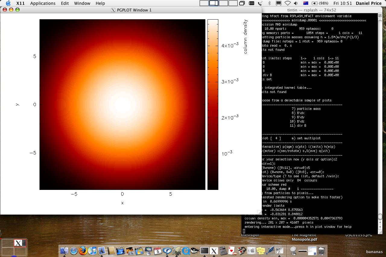
Fig. 2 Screenshot of 3D column density plot to an X-window
Important
Rendered plots only work if columns for density, particle mass and smoothing length are correctly identified in the data, and provided the number of coordinates is 2 or greater. Without these, rendering will just colour the points according to the selected column. See Data reads and command line options for internal details.
Cross section
To plot a cross section slice instead of a projection in 3D, simply
use --xsec flag on the command line:
splash --xsec -r 5 minidump.00001
Or, type x at
the main menu to open the (x) cross section/3D plotting options and
choose option 1) switch between cross section and projection. Then
re-plot the rendered plot again (exactly as in the previous example
Rendered plots), setting the slice position at the prompt:
enter z position for cross-section slice: ([-8.328:8.327], default=0.000):
which produces the plot shown in the screenshot in Fig. 3
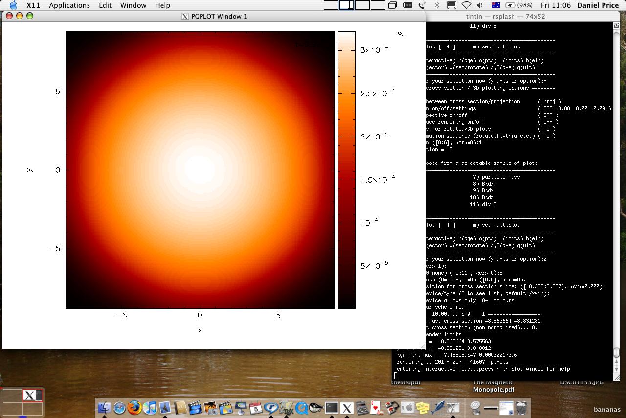
Fig. 3 Screenshot of 3D Cross section slice plot to an X-window
Vector plots
A prompt to plot vector arrows on top of Rendered plots (or on top of particle plots) appears whenever vectors are present in the data (for details of how to specify this in your data read, see Data reads and command line options), taking the form:
(vector plot) (0=none, 8=B) ([0:8], default=0):0
where the number refers to the column of the first component of the vector quantity.
Vector plots in 3D show either the integral of each component along the line of sight or, for a Cross section, the vector arrows in a Cross section slice (depending on whether a projection or Cross section has been selected for 3D plots – see the rendering examples given previously). In 2D vector plots simply show the vector arrows mapped to a pixel array using the SPH kernel.
Settings related to vector plots can be changed via (v)ector plot options.
The size of the arrows is set by the maximum plot limit over all of the vector components.
Alternatively the arrow size can be changed interactively using v, V (decrease
/increase the arrow size) and w (automatically
adjust arrow size so longest arrow is one pixel width).
Contour plots
To plot contours of a quantity instead of Rendered plots, simply set the colour scheme used for rendering to 0 (contours only) via the “change colour scheme” option in the (r)endering options (type “r2” from the main menu as a shortcut to option 2 in the (r)endering options).
Contours of an additional quantity can also be plotted on top of
Rendered plots. However the prompt for an additional contour plot does not
appear by default – it can be turned on via the plot contours option
in the (r)endering options (type r3 at the main menu as a shortcut). With
this option set and a non-zero response to the render prompt, a prompt
appears below the render prompt:
(render) (0=none) ([0:11], default=0):5
(contours) (0=none) ([0:11], default=0):6
Entering the column to use in the contour plot at this prompt (e.g. column 6 in the above example would correspond to the temperature) gives a rendered plot with overlaid contours.
Entering the same quantity used in the rendering at this prompt (e.g.
column 5 in the above example) triggers a subsequent prompt for the
contour limits which can then be set differently to those used in the
render plot. In this way it is possible to make a plot where the density
of one particle type is shown by the rendered plot and the density of
another particle type (with different limits) is shown by contours. This
can be achieved because once contour plotting is turned on, the
contribution of a given particle type to either the contours or rendered
plots can be turned on or off via the turn on/off particles by type
option in the particle plot (o)ptions.
Moving forwards and backwards through data files
See Interactive mode. If you have put more than one file on the command line (or alternatively the file contains more than one dump), it is then possible to move forwards and backwards through the data:
press the
space barto move to the next file (with the cursor in the plot window - this is Interactive mode).press
bto load and plot the previous filetype 9 and press
spaceto move forward by 9 filestype 10 and press
bto move back by 10 files
Press h in Interactive mode for more.
Important
If you plot to a non-interactive device, splash simply cycles through all the files on the command line automatically.
Zooming in and out / changing plot limits
See Interactive mode. Having plotted to an interactive device (e.g. /xw), tasks such as
zooming in and out, selecting, colouring and hiding particles, changing
the limits of both the plot and the colour bar and many other things can
be achieved using either the mouse (i.e., selecting an area on which to
zoom in) or by a combination of the mouse and a keystroke.
Producing figures for LaTeX documents
Producing a pdf or postscript plot suitable for inclusion in a LaTeX file is simple. At the device prompt, type
Graphics device/type (? to see list, default /xw): myfile.eps
that is, instead of /xw (for an X-window), simply type /eps or
.eps to use the encapsulated postscript driver. This produces a file
which by default is called splash.eps, or if multiple files have
been read, a sequence of files called splash_0000.eps,
splash_0001.eps, etc. To specify both the device and filename, type
the full filename (e.g. myfile.eps) as the device. Files produced in
this way can be directly incorporated into LaTeX using standard packages.
Danger
Do not use the /png driver to produce files for LaTeX documents. Your
axes will appear pixellated and blurred.
Use a vector graphics device (eps or pdf) instead. These give clean, sharp
and infinitely scalable text and lines.
Hint
Using eps format is recommended for LaTeX as it will always crop
to the exact boundaries of the plot. The inbuilt pdf driver may
require cropping of whitespace. Encapsulated postscript can be easily
converted to pdf (for pdflatex) on the command line using:
epstopdf file.eps
Most pdflatex engines (including Overleaf) will handle/convert eps automatically.
Producing a movie of your simulation
To make a movie of your simulation, first specify all of the files you want to use on the command line:
splash dump_*
and use an interactive device to adjust options until it looks right.
Hint
Movies look best with minimal annotation, e.g. using Hollywood mode or the backspace key in interactive mode to manually delete annotation
If in interactive mode type s to save the current settings, then plot the
same thing again but to a non-interactive device.
In the latest version of splash you can generate an mp4 directly
Graphics device/type (? to see list, default /xw): splash.mp4
In older splash versions, or for more control, first generate a sequence of png files
Graphics device/type (? to see list, default /xw): /png
This will generate a series of images named splash_0000.png,
splash_0001.png, splash_0002.png corresponding to each new
plotting page generated (or enter “myfile.png” at the device prompt
to generate myfile_0000.png, myfile_0001.png,
myfile_0002.png…).
Hint
Avoid prompts altogether using the Command line options. For example, to make a movie as per the prompts above, simply type:
splash -r 5 --movie dump_*
which is a shortcut for:
splash -r 5 -dev splash.mp4 dump_*
To produce a sequence of images from the command line, use
splash -r 5 -dev /png
See also Reading/processing data into images without having to answer prompts.
Producing a movie from a sequence of images
Having obtained a sequence of images there are a variety of ways to make these into an animation using both free and commercial software. The simplest is to use ffmpeg:
ffmpeg -i splash_%04d.png -r 10 -vb 50M -bt 100M -pix_fmt yuv420p -vf setpts=4.*PTS movie.mp4
A simple script which executes the above command is included in the source file distribution
~/splash/scripts/movie.sh
Alternatively, it is possible to create an animation from a list of image files:
ffmpeg -f concat -r 25 -i list.txt -vb 50M -bt 100M -vcodec mpeg4 -vf setpts=4.*PTS movie.mp4
Where list.txt contains the image files you want to use like this:
file 'path/to/file1.png'
file 'path/to/file2.png' etc
See How do I make a movie from splash output? for more.
Hollywood mode
Press Enter or ctrl-m in the interactive plot window to start Hollywood mode,
which changes to plot settings better suited to movies.
The following shows A circumbinary disc simulation viewed in default mode:
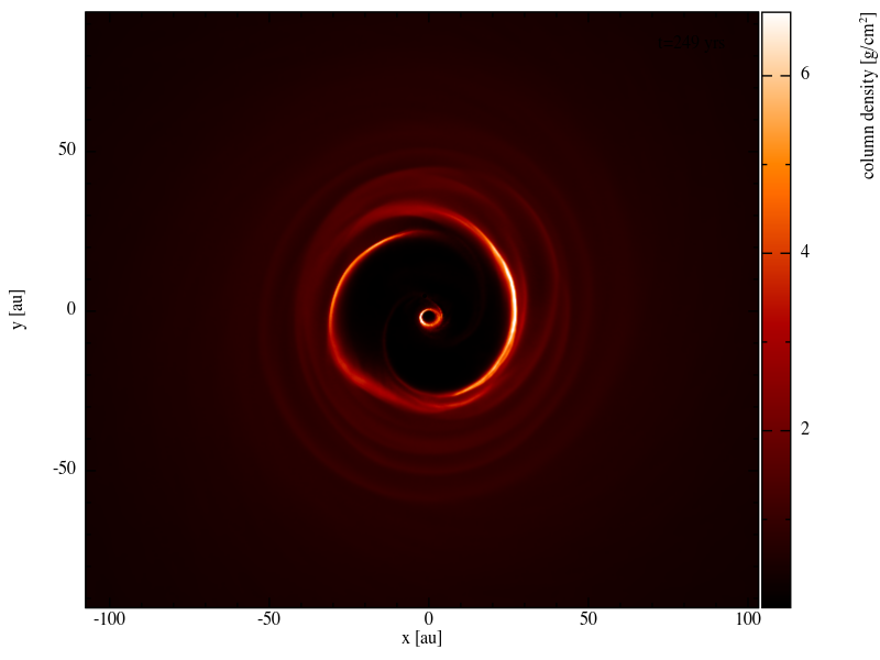
Fig. 4 A circumbinary disc simulation viewed in default mode
and The same simulation viewed in Hollywood mode
Fig. 5 The same simulation viewed in Hollywood mode
Remote visualisation
Visualisation of data in-situ on a cluster or supercomputer is simple. Just log in using ssh with X-windows forwarding, e.g.:
ssh -Y dprice@gadi.nci.org.au
Then just plot to an interactive device (/xw) as usual and everything
in Interactive mode should just work.
splash has few dependencies and is simple to install in your home space if necessary. That said, it is always a good idea to get admins to install a shared package for all users.
Ten quick hints for producing good-looking plots
These can improve the look of a visualisation substantially compared to the default options:
Log the colour bar. To do this simply move the cursor over the colour bar and hit
l(for log) in Interactive mode. Or non-interactively via theapply log or inverse transformations to columnsoption in the (l)imits menu.Adjust the colour bar limits. Position the mouse over the colour bar and left-click in Interactive mode. To revert to the widest max/min possible for the data plotted, press
awith the cursor positioned over the colour bar. Limits can also be set manually in the (l)imits menu.Change the colour scheme. Press
morMin Interactive mode to cycle forwards or backwards through the available colour schemes.Change the paper size. To produce high-resolution images/movies, use the
change paper sizeoption in the (p)age options to set the paper size in pixels.Try normalised or exact interpolation. If your simulation does not involve free surfaces (or alternatively if the free surfaces are not visible in the figure), turning the
normalise interpolationsoption on (in the (r)endering options) may improve the smoothness of the rendering. This is turned off by default because it leads to funny-looking edges. Exact rendering performs exact sub-pixel rendering so is more accurate but slower.Remove annotation/axes. For movies, often axes are unnecessary and detract from the visual appeal. Use Hollywood mode or delete annotation by pressing backspace in Interactive mode. Alternatively each can be turned off manually – axes via the
axes optionsoption in the (p)age options; the colour bar by thecolour bar optionsentry in the (r)endering options and the legends via options in the le(g)end and title options.Change axes/page colours. The background colour (colour of the page) and foreground colour (used for axes etc) can be changed vie the
set foreground/background coloursoption in the (p)age options.Move the legend or turn it off. The time legend can be moved by positioning the mouse and pressing
Gin interactive mode. The legend can be turned off in the le(g)end and title options or by pressing backspace in interactive mode. Similarly the vector plot legend can be turned on/off in the (v)ector plot options and moved by positioning the cursor and pressingH.Use physical units on the axes. These can be set via the (d)ata options. See Changing physical unit settings for more details.
Save settings to disk! Don’t waste your effort without being able to reproduce the plot you have been working on. Pressing
sin interactive mode only saves the current settings for subsequent timesteps. Pressingsfrom the main menu saves these settings to disk. PressingSfrom the main menu saves both the plot options and the plot limits, so that the current plot can be reproduced exactly when splash is next invoked. Adding ana, as inSA,Saorsato the save options gives a prompt for a different prefix to the filenames (e.g.splash.defaultsbecomesmyplot.defaults), which splash can be invoked to use via the-pcommand line option (e.g.splash -p myplot file1 file2...).